"It's not whether you're right or wrong, but how much money you make when you're right and how much you lose when you're wrong."
— George Soros
Today’s piece comes as a result of premium members requesting an exploration into the concepts I use to run my one-man-insurance-company and separate myself from the gamblers.
In it we cover the concepts of a mathematical edge and how to calculate it, as well as the Kelly criterion and its use in calculating the correct position sizing for a trading portfolio.
Do You Have an Edge?
First thing’s first.
Before taking on any trade —especially any binary trade such as credit spreads—the first checkpoint is to ascertain whether or not a profit is to be expected if it were to be made many times in total.
Edge has a precise definition. It is the degree to which your expected return on a bet exceeds what a fair, zero-sum game would offer.
I tend to refer to Expected value (EV) which is the mathematical expression of that edge applied to a specific trade. It is what you calculate when you plug your probabilities and payoffs into the formula. EV is how you measure edge and is calculated thusly:
EV = (p × b) − (q × l)
p = probability of winning
b = payoff per dollar risked
q = probability of losing (1 − p)
l = fraction of stake lost on a losing trade (binary outcome = 1; options trade residual value = <1)
Real Example From The Vault
GLD Feb27 415/410 Bull P
On 2/2/2026, GLD was trading around $430.
I informed members that I was selling a bull put spread, where I sold put option at the $415 strike and bought put options at the $410 strike in equal amounts, with both contracts expiring on Feb27, 2026. For every 1 spread sold, I received an upfront payment of $108 (my max profit, realized if GLD finished above $415 by expiration) with a potential max loss of $392 (if GLD were to finish below $410 by expiration)
The probability of the trade finishing in max profit was calculated at 78.4% via the Black Scholes formula.
Calculating the EV:
EV = (p × b) − (q × l)
p = 0.784 (market-implied probability of full profit)
b = 0.276 (premium collected $108 ÷ max loss $392 — payoff per dollar risked)
q = 0.216 (1 − p)
l = 1 (full max loss if breached)
(0.784 × 0.276) − (0.216 × 1) = 0.216 − 0.216 = ~0.00
This makes sense - the options are fairly priced so one should expect a positive nor negative EV.
A VERY important note - The EV for most binary options trades will actually be zero or negative thanks to the market arbitraging away most obvious edges over the years. This assumes a trader lets the trade expire worthless (total loss). The EV can often be flipped positive via certain stop loss rules (shared with premium members) as it significantly reduces the max loss, allowing the trade to be rolled forward maintaining a positive EV.
Putting this into practice let’s return to my trade on GLD above, but change one variable, I set a strict stop loss to 150% of the credit I received upfront for putting on the trade.
Credit received: $108
Max loss (stop): $108 × 1.5 = $162 per contract (vs $392 without stop)
At market-implied p = 0.784, the EV now resembles the following.
(0.784 × 0.276) − (0.216 × 0.413) = 0.216 − 0.089 = EV of $0.127 per dollar risked
On $392 capital at risk: ~$49.68 edge per contract
An edge can also be obtain through various factors and lateral thinking, one of which includes the timing of selling options for credit —as in this example— when implied volatility is higher than the historic norm. This has the effect of increasing the probability of profit and boosting the EV.
Philosophically, edge is repeatable and structural and EV is situational.
If you’ve made it this far, congratulations, you’ve done more than most and moved from the gambler speculator mindset to that of the professional trader.
The question now is: given that I have an edge, how much of my working capital should I risk to maximise profits without blowing up my bankroll?
The Kelly Criterion
That question actually has a quite a answer. It was discovered in 1956 by a Texan researcher named John L. Kelly Jr.

Interesting cat. Rather flamboyant by most accounts. He was working on information theory and noise on telephone lines while working at Bell labs and also studied the performance of gamblers betting on horse races.
If a gambler could determine an edge, Kelly sought to mathematically determine the exact fraction of a bankroll to wager per bet to maximize the long-term bank roll growth while avoiding bankruptcy.
A lesser known fact I love; Kelly also found that the performance of gamblers at the race track worsened in proportion to the “information” they received. Now consider the tsunami of macro-shmacro content the dominates the financial media and consider its value to investor performance..
The formula he discovered is written as:
f* = (bp − q) / b
Applying the formula to my GLD trade above (with stop loss)
b = payoff per dollar risked = $108 ÷ $162 = 0.667
p = probability of winning = 0.784 (market-implied)
q = probability of losing = 0.216
f* = optimal fraction of bankroll to stake
= (0.667 × 0.784 − 0.216) / 0.667 = 0.460
Full Kelly says 46% of bankroll. Half Kelly: 23%.
Note: this assumes only running one type of trade at a time, repeated many times, and full Kelly requires balls of steel to trust the math.
One also needs to update their bankroll as it grows or shrinks for calculating % allocation. Ie. I seeded Machina in January, 2026 with $50k. Realised profits now make the capital $61,916. Ergo, using full Kelly as above I’d now need calculate 46% of $61.9K, rather than $50K as I would’ve in Jan.
Unfortunately John Kelly died of a stroke on a Manhattan footpath at age 41. He reportedly smoked 6 packs of cigarettes a day and never got to put his Criterion to work.
Enter Ed Thorp
The man who did put Kelly’s theory into practice was Edward O. Thorp - Polymath and a personal hero of mine. Beat the Dealer is the founding document of quantitative finance dressed as a blackjack book. Thorp applied the Kelly criterion to various gambling games and cleaned out casinos. He then started a hedge fund, pioneering warrant hedging, convertible bonds arbitrage in the stock market decades before quant investing had a name. His work has a heavy influence in the way I ran my Machina.
The Purpose Of The Kelly Criterion
Avoiding bankruptcy.
EV tells me whether to take the bet / place the trade.
The Kelly Criterion tells me how much to put behind it.
And Overbetting is much worse than underbetting.
Under-betting in Kelly terms means growing the bankroll more slowly while avoiding ruin.
Over-betting however causes the variance to expand until you cross a critical threshold Kelly’s paper calls f_c, beyond which ruin is mathematically inevitable regardless of your edge
The formula is free. The edge is yours to find. The only question left is whether you will size correctly when you have one, or whether you will do what most traders do — “got a hunch, bet a bunch” and over-bet, then wonder why they blow up.
In the next piece I go deeper into Monte Carlo simulation and how to stress-test the repeatability of an edge across thousands of simulated trades before risking a dollar. If Kelly tells how much to bet, Monte Carlo tells whether your edge survives contact with reality.
Premium members receive full access to every trade I put on inside Machina Capitalis: entry, sizing, stop levels, and the EV calculation behind each position. Everything above, applied in real time.
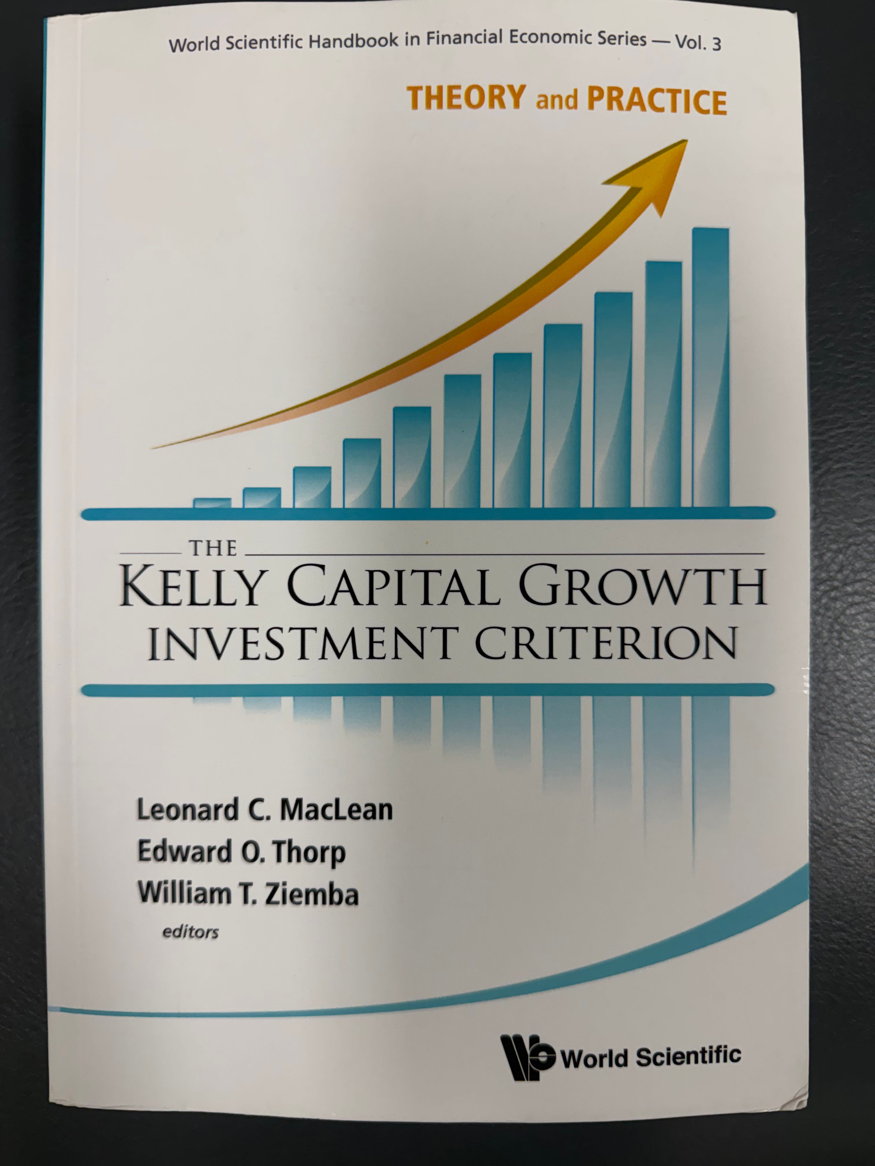
If this resonated, forward it to someone who still thinks position sizing is a round number they feel comfortable with.
All the best,
— Benjamin
This article draws on “The Kelly Criterion and the Stock Market” by Louis M. Rotando and Edward O. Thorp, published in The American Mathematical Monthly, Vol. 99, No. 10, December 1992.
Kelly, J. L., Jr. (1956). A new interpretation of information rate. Bell System Technical Journal, 35(4), 917–926.